Non-linear Soybean Growth
 Image credit: VectorStock
Introduction
The data in this study were collected in the Department of Crop Sciences at North Carolina State University and utilized in Davidian (n.d.). The objective of the study is to compare the growth curve of two soybean genotypes, Forrest (F) and Plant Introduction (P). Forest is a common commercial variety wherease Plant Introduction is an experimental strain. There are a total of 48 plants contained in the dataset with 8 to 10 average leaf weight per plant (g) taken at weekly increments. According to Davidian (n.d.), “At each sampling time, 6 plants were randomly selected from each plot, leaves from these plants were mixed together and weighted, and an average leaf weight per plant (g) was calcuated.” The summary of the average leaf weight per plant is shown in Table 1.
| Variable | N | Mean | Minimum | Maximum |
|---|---|---|---|---|
| Forrest (F) | 204 | 5.120 | 0.029 | 21.810 |
| Plant Introduction (P) | 208 | 7.196 | 0.063 | 30.272 |
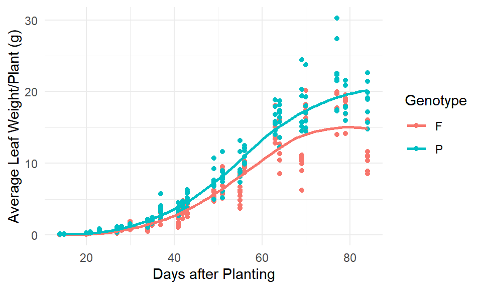
Figure 1: Visual display of soybean growth by genotype.
Soybeans tend to grow at a slower rate at the beginning of the season and then increase their growth rate until leveling off at the end of the season. This sigmoidal or S-shaped pattern is shown in the Figure 1. The proposed non-linear function to fit the given data as a growth curve is the logistic growth model. We will consider both the three parameter model where
\[ W(x;\boldsymbol\theta) = \frac{a}{1+be^{-cx}} \] as well as the four parameter model where
\[ W(x;\boldsymbol\theta) = a + \frac{b - a}{1+e^{(c-x)/d}} \]
For each of the models above, \(x\) is the number of days after planting, and starting values for \(\boldsymbol\theta\) will be determined according to the initial and asymptotic average leaf weight per plant. We will determine the whether the 4-parameter logistic model is necessary by comparing Model (1) to Model (2) using likelihood ratios. After the correct model has been selected, we will compare the two genotypes and account for nonconstant variance. Finally, using NLMIXED in SAS, we will account for the within individual variation.
Model Selection
In Model (1), \(a\) is defined as the asymptotic weight, while \(\frac{a}{1+b}\) is the initial weight, and \(c\) determines the growth rate. Selecting starting values of \(\hat{\boldsymbol\theta}=(20,700,0.125)^T\) and assuming the errors are normally distributed with constant variance, we fit Model (1) using OLS (ordinary least squares) in the NLS function found in the Stat pakcage. We obtain \(\hat\sigma^2 = 5.13\) and parameter estimates provided in Table 2.
| Estimate | Std. Error | |
|---|---|---|
| a | 18.418 | 0.436 |
| b | 748.074 | 248.403 |
| c | 0.123 | 0.007 |
In Model (2), \(b\) is defined as the asymptotic weight, \(a\) is used in defining the initial weight, and \(c\) and \(d\) determine the growth rate. Selecting starting values of \(\hat{\boldsymbol\theta} = (0.2, 20, 50,8)^T\) and assuming the errors are normally distributed with constant variance, we obtain \(\hat\sigma^2 = 5.13\) and parameter estimates provided in Table 3.
| Estimate | Std. Error | |
|---|---|---|
| a | 0.181 | 0.243 |
| b | 18.313 | 0.456 |
| c | 54.073 | 0.677 |
| d | 7.865 | 0.609 |
Using extra sum of squares analyses to comparing Model (1) to Model (2), we obtain an F-ratio of 0.51 (p-value 0.48) and conclude the 3-parameter logistic model captures the growth pattern adequately. This is also verified conceptually since the initial leaf weight of plants is 0, and thus the extra parameter is unnecessary to capture this value.
| Res.Df | Res.Sum Sq | Df | Sum Sq | F value | Pr(>F) |
|---|---|---|---|---|---|
| 409 | 2096.80 | NA | NA | NA | NA |
| 408 | 2094.16 | 1 | 2.63 | 0.51 | 0.47 |
Evaluating Model (1), we can see there are nonconstant variance issues due to the fanning out of residuals as well as the possibility of differing parameters between genotypes.
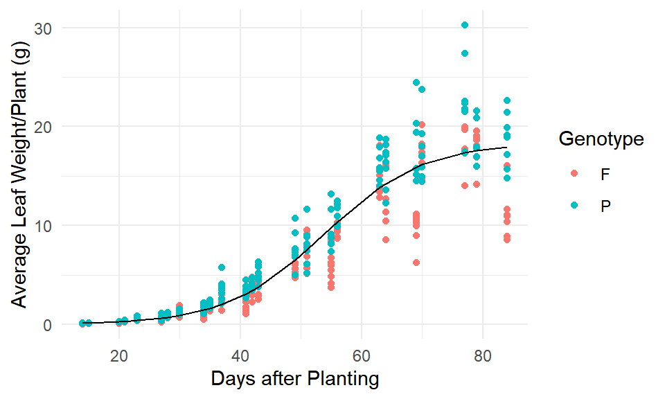
(#fig:mod1_fit)Model (1) fit
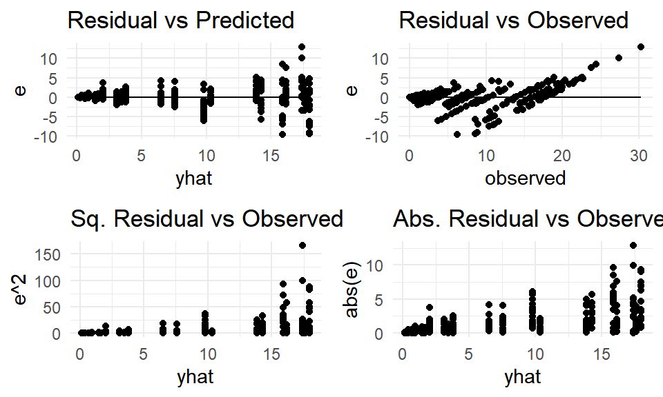
(#fig:mod1_resid)Model (1) residuals
Growth Pattern due to Genotype
Define the indicator variable,
\[Genotype\_P=\begin{cases} 1 & Genotype = P \\ 0 & Genotype \ne P. \end{cases}\]
Consider incremental parameters, \(ap, bp,\) and \(cp\) accounting for the change in the parameter between the two genotypes. Starting values were selected by first fitting Model (1) to each genotype individually to obtain \(\hat{\boldsymbol\theta} = (16, 4.78, 1035, -490,0.125, -0.01)^T\). Fitting the full model,
\[\begin{equation} W(x;\boldsymbol\theta) = \frac{a+ap\cdot Genotype\_P}{1+(b+bp\cdot Genotype\_P)e^{-(c+cp\cdot Genotype\_P)x}} \end{equation}\]
we obtain parameter estimates in Table 4.
| Estimate | Std. Error | |
|---|---|---|
| a | 16.037 | 0.516 |
| ap | 4.786 | 0.781 |
| b | 1035.567 | 531.486 |
| bp | -489.899 | 563.531 |
| c | 0.129 | 0.011 |
| cp | -0.013 | 0.013 |
Since we are unsure whether each of these incremental parameters are necessary, we will use extra sums of squares to determine the best fit. Fitting
\[\begin{equation} W(x;\boldsymbol\theta) = \frac{a}{1+(b+bp\cdot Genotype\_P)e^{-(c+cp\cdot Genotype\_P)x}}, \end{equation}\]
and comparing Model (4) to Model (3), we conclude with an F value of 37.62 and p-value < 0.0001 that the incremental parameter, \(ap\) is necessary to keep in the model.
| Res.Df | Res.Sum Sq | Df | Sum Sq | F value | Pr(>F) |
|---|---|---|---|---|---|
| 407 | 1786.25 | NA | NA | NA | NA |
| 406 | 1634.77 | 1 | 151.47 | 37.62 | 0 |
Fitting,
\[\begin{equation} W(x;\boldsymbol\theta) = \frac{a+ap\cdot Genotype\_P}{1+(b)e^{-(c+cp\cdot Genotype\_P)x}}, \end{equation}\]
and comparing Model (5) to Model (3), we conclude with an F value of 1.24 and p-value of 0.27 that the incremental parameter \(bp\) is not necessary to keep in the model.
| Res.Df | Res.Sum Sq | Df | Sum Sq | F value | Pr(>F) |
|---|---|---|---|---|---|
| 407 | 1639.78 | NA | NA | NA | NA |
| 406 | 1634.77 | 1 | 5 | 1.24 | 0.27 |
Fitting \[\begin{equation} W(x;\boldsymbol\theta) = \frac{a+ap\cdot Genotype\_P}{1+(b)e^{-(c)x}}, \end{equation}\]
and comparing Model (6) to Model (5), we conclude with an F value of 0.04 and p-value of 0.84 that the incremental parameter \(cp\) is not necessary to keep in the model.
| Res.Df | Res.Sum Sq | Df | Sum Sq | F value | Pr(>F) |
|---|---|---|---|---|---|
| 408 | 1639.93 | NA | NA | NA | NA |
| 407 | 1639.78 | 1 | 0.16 | 0.04 | 0.84 |
After comparing models, we conclude that Model (6), the 3-parameter logistic model with an incremental parameter due to genotype for parameter a, is the best fit. The estimated paramters are shown in Table 8 and the fitted values grouped by genotype are shown in Figure 4.
| Estimate | Std. Error | |
|---|---|---|
| a | 16.291 | 0.411 |
| ap | 4.273 | 0.409 |
| b | 695.142 | 199.701 |
| c | 0.121 | 0.006 |
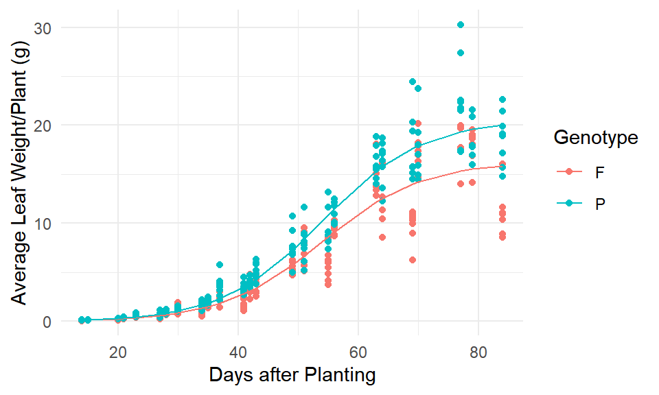
(#fig:mod6_fit)Model (6) fit.
Evaluating the residuals from Model (6), there is clear indication of nonconstant variance due to the fanning out of residuals.
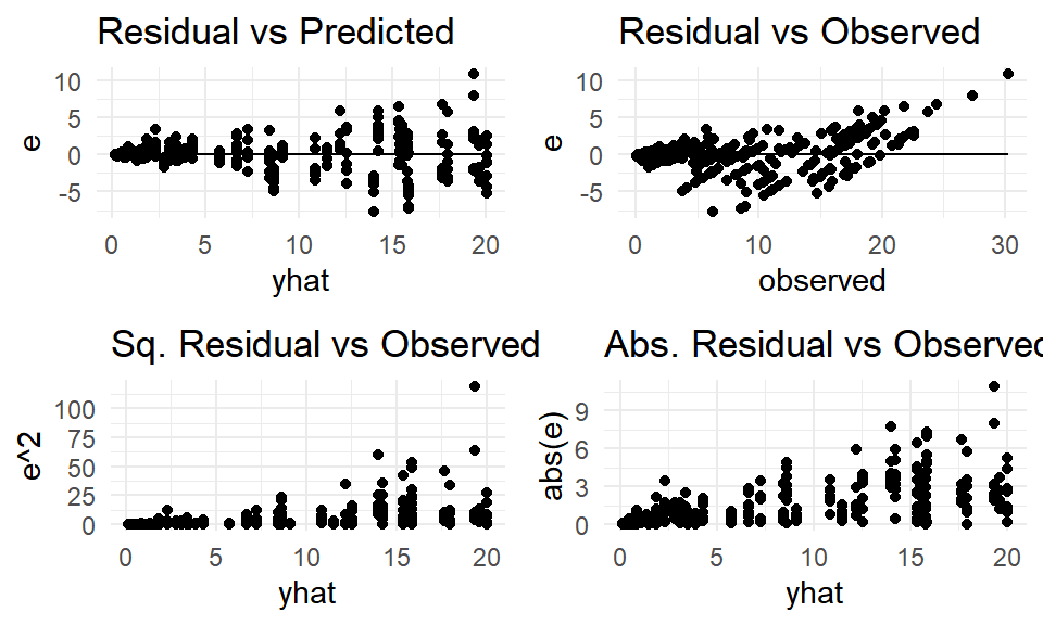
(#fig:mod6_resid)Model (6) residuals.
Fitting Model (6), we now assume nonconstant variance and are not necessarily restricted to normally distributed errors. In particular, we model the variance using a function of \((f(x_i|\boldsymbol\theta), \psi\), and other constants \(z_i\). In general, \(Var(y_i) = \sigma^2g^2(\theta,\psi,z_i).\) Using GLS (generalized least squares) to estimate weights, we obtain \(\psi = 0.88\) and parameter estimates in Table 9.
| Estimate | Std.Error | |
|---|---|---|
| a | 14.975 | 0.246 |
| ap | 4.739 | 0.395 |
| b | 905.667 | 21.049 |
| c | 0.131 | 0.001 |
Observing the studentized residuals produced by assuming nonconstant variance, we still determine there appears to be more going on. One possibility is the variability between plots.
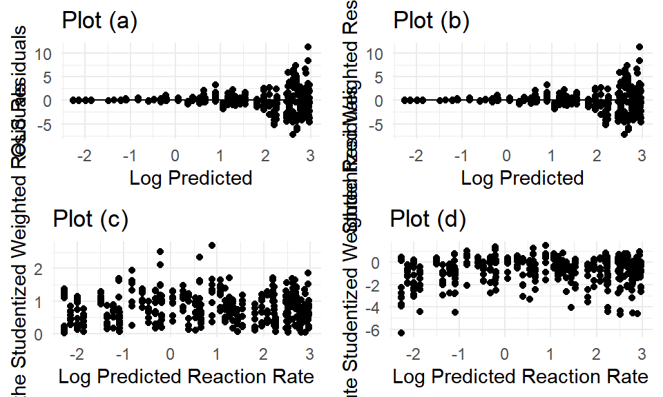
(#fig:mod7_diagnostics)Model (7) residuals.
Experimental Design
The variability between plants may be affecting the model. We can accounting for this using a Nonlinear Mixed Effects Model. We will fit Model 6 assuming error terms that are normally and independently and identically distributed as well as a random effect, \(a_i\), accounting for the variation due to the plot at the asymptotic leaf weight. Using NLMIXED in SAS, we obtain parameter estimates of,
##                               Random Effects
##
##                            The NLMIXED Procedure
##
##                            Parameter Estimates
##
##                      Standard                             95% Confidence
## Parameter  Estimate     Error    DF  t Value  Pr > |t|        Limits
##
## a           14.9235    0.8175    47    18.26    <.0001   13.2790   16.5680
## ap           5.2961    1.0833    47     4.89    <.0001    3.1168    7.4753
## b            937.69   51.6136    47    18.17    <.0001    833.85   1041.52
## c            0.1314  0.002038    47    64.47    <.0001    0.1273    0.1355
## s2ai        12.1721    2.9228    47     4.16    0.0001    6.2922   18.0520
## s2          0.05810  0.005236    47    11.10    <.0001   0.04757   0.06863
## psi          0.9296   0.02791    47    33.31    <.0001    0.8735    0.9857
##
##                             Parameter Estimates
##
##                             Parameter  Gradient
##
##                             a          0.000145
##                             ap         -0.00003
##                             b          2.066E-6
##                             c          -0.02470
##                             s2ai       -0.00003
##                             s2         0.009738
##                             psi        0.001264
Conclusion
Overall, the 3-parameter model with an incramental parameter to capture the varying asymptotic weights between genotypes and a random effect due to the plot variation is the best selection for modeling the leaf weight per plant (g) of soybeans over the days after planting. From the final model, the estimated asymptotic weight for a soybean with the Forrest (F) genotype is 14.92 g and for a soybean with the Plant Introduction (P) genotype is 20.22 g.
Code Appendix
library(knitr)
library(dplyr)
knitr::opts_chunk$set(echo = TRUE)
knitr::opts_chunk$set(fig.width=7, fig.height=6, fig.align = "center")
knitr::opts_chunk$set(tidy.opts=list(width.cutoff=50),tidy=TRUE)

library(SASmarkdown)
sas_enginesetup(sashtml=sashtml)
sasexe <- "C:/Program Files/SASHome/SASFoundation/9.4/sas.exe"
sasopts <- "-nosplash -ls 75"

resid_panel <- function(data = data, yhat = yhat, observed = y){
  require(ggplot2)
  require(gridExtra)
  e = observed - yhat
  resid1 <- ggplot(data, aes(x = yhat, y = e)) +
    geom_point() +
    geom_line(aes(y = 0)) +
    theme_minimal() +
    ggtitle("Residual vs Predicted")

  resid2 <- ggplot(data, aes(x = observed, y = e)) +
    geom_point() +
    geom_line(aes(y = 0)) +
    theme_minimal() +
    ggtitle("Residual vs Observed")

  resid3 <- ggplot(data, aes(x = yhat, y = e^2)) +
    geom_point() +
    theme_minimal() +
    ggtitle("Sq. Residual vs Observed")

  resid4 <- ggplot(data, aes(x = yhat, y = abs(e))) +
    geom_point() +
    theme_minimal() +
    ggtitle("Abs. Residual vs Observed")

  grid.arrange(resid1, resid2, resid3, resid4, ncol = 2)
}

corr_panel <- function(data = data2, x = x, e = e){
  require(ggplot2)
  require(gridExtra)

  corr_1 <- ggplot(data = data, aes(x = x, y = e)) +
    geom_point() +
    geom_smooth(se = F) +
    geom_line(aes(y = 0)) +
    theme_minimal() +
    ggtitle("Distance vs Residual")

  corr_2 <- ggplot(data = data, aes(x = lag(e), y = e)) +
    geom_point() +
    geom_smooth(se = F) +
    geom_line(aes(y = 0)) +
    theme_minimal() +
    ggtitle(paste("Nth Residual vs (N-1)st Residual: \n Corr = ", round(cor(lag(e)[-1],e[-1]),4))) +
    xlab("lag1_e")
  corr_2

  corr_3 <- ggplot(data = data, aes(x = lag(lag(e)), y = e)) +
    geom_point() +
    geom_smooth(se = F) +
    geom_line(aes(y = 0)) +
    theme_minimal() +
    ggtitle(paste("Nth Residual vs (N-2)nd Residual: \n Corr = ", round(cor(lag(lag(e))[-c(1:2)],e[-c(1:2)]),4), sep = "")) +
    xlab("lag2_e")

  corr_4 <- ggplot(data = data, aes(x = lag(lag(lag(e))), y = e)) +
    geom_point() +
    geom_smooth(se = F) +
    geom_line(aes(y = 0)) +
    theme_minimal() +
    ggtitle(paste("Nth Residual vs (N-3)rd Residual: \n Corr = ", round(cor(lag(lag(lag(e)))[-c(1:3)],e[-c(1:3)]),4), sep = "")) +
    xlab("lag3_e")

  grid.arrange(corr_1, corr_2, corr_3, corr_4, ncol = 2)

}

studentized_resid_panel <- function(data = data, yhat = yhat, residual = residual, studentized_residual = studentized_residaul){
  plota <- ggplot(data, aes(x = log(yhat), y = residual)) +
      geom_point() +
      geom_line(aes(y = 0)) +
      theme_minimal() +
      xlab("Log Predicted") +
      ylab("OLS Residuals") +
      ggtitle("Plot (a)")

    plotb <- ggplot(data, aes(x = log(yhat), y = residual)) +
      geom_point() +
      geom_line(aes(y = 0)) +
      theme_minimal() +
      xlab("Log Predicted") +
      ylab("Studentized Weighted Residuals") +
      ggtitle("Plot (b)")

    plotc <- ggplot(data, aes(x = log(yhat), y = (studentized_residual^2)^(1/3))) +
      geom_point() +
      theme_minimal() +
      xlab("Log Predicted Reaction Rate") +
      ylab("2/3 root of the Studentized Weighted Residuals") +
      ggtitle("Plot (c)")
    coef(lm((studentized_residual^2)^(1/3) ~ log(yhat)))

    plotd <- ggplot(data, aes(x = log(yhat), y = log(abs(studentized_residual)))) +
      geom_point() +
      theme_minimal() +
      xlab("Log Predicted Reaction Rate") +
      ylab("Log Absolute Studentized Weighted Residuals") +
      ggtitle("Plot (d)")
    coef(lm(log(abs(studentized_residual)) ~ log(yhat)))

    grid.arrange(plota, plotb, plotc, plotd, ncol = 2)
    }
    soybean_data <- read.csv("Data/soybean_data.csv")
    cols <- c(1,3)
    soybean_data[cols]  <- lapply(soybean_data[cols], factor)
    Fsum <- summary(soybean_data[soybean_data$Genotype == "F",])
    Psum <- summary(soybean_data[soybean_data$Genotype == "P",])

    data_sum <- data.frame("Variable" = c("Forrest (F)", "Plant Introduction (P)"),
                           "N"        = c(204,208),
                           "Mean"     = c(5.12,7.196),
                           "Minimum"  = c(0.029,0.063),
                           "Maximum"  =c(21.81,30.272))
    kable(data_sum, caption = "Summary of average weight per plant (g)")
    library(ggplot2)
    ggplot(soybean_data, aes(x = Days, y = Leaf_Weight, group = Genotype, color = Genotype)) +
      geom_point() +
      geom_smooth(se = F) +
      theme_minimal() +
      xlab("Days after Planting") +
      ylab("Average Leaf Weight/Plant (g)")

mod1 <- nls(Leaf_Weight ~ a/(1+b*exp(-c*Days)),
                 data = soybean_data,
                 start = list(a = 20, b = 700,c = 0.125))
#summary(mod1)$sigma^2
kable(round(summary(mod1)$coeff[,1:2],3), caption = "Estimated parameters for Model (1)")
mod2 <- nls(Leaf_Weight ~ a + (b-a)/(1+exp((c-Days)/d)),
            data = soybean_data,
            start = list(a = 0.2, b = 20,c = 50, d = 8))
# summary(mod2)$sigma^2
kable(round(summary(mod2)$coeff[,1:2],3), caption = "Estimated parameters for Model (2)")
kable(round(anova(mod1, mod2),2), caption = "Extra sum of squares model (1) vs model (2)")
    ggplot(soybean_data, aes(x = Days, y = Leaf_Weight, group = Genotype, color = Genotype)) +
      geom_point() +
      geom_line(aes(y = fitted(mod1)), color = "black") +
      theme_minimal() +
      xlab("Days after Planting") +
      ylab("Average Leaf Weight/Plant (g)")
resid_panel(data = soybean_data, yhat = fitted(mod1), observed = soybean_data$Leaf_Weight)
library(fastDummies)
soybean_data2 <- soybean_data[order(soybean_data$Genotype),]
soybean_data2 <- dummy_cols(soybean_data2, select_columns = "Genotype", remove_first_dummy = TRUE)
mod3 <- nls(Leaf_Weight ~ (a+ap*Genotype_P)/(1+(b+bp*Genotype_P)*exp(-(c+cp*Genotype_P)*Days)),
            data = soybean_data2,
            start = list(a = 16, ap = 4.78, b = 1035, bp = -490, c = 0.125, cp = -0.01))
kable(round(summary(mod3)$coeff[,1:2],3), caption = "Estimated parameters for Model (3)")
# Take away ap? No
mod4 <- nls(Leaf_Weight ~ (a)/(1+(b+bp*Genotype_P)*exp(-(c+cp*Genotype_P)*Days)),
            data = soybean_data2,
            start = list(a = 20, b = 1035, bp = -490, c = 0.125, cp = -0.01))
kable(round(anova(mod4, mod3),2), caption = "Extra sum of squares model (4) vs model (3)")
# Take away bp? Yes
mod5 <- nls(Leaf_Weight ~ (a + ap*Genotype_P)/(1+(b)*exp(-(c+cp*Genotype_P)*Days)),
            data = soybean_data2,
            start = list(a = 16, ap = 4.78, b = 700, c = 0.125, cp = -0.01))
kable(round(anova(mod5, mod3),2), caption = "Extra sum of squares model (5) vs model (3)")
# Take away cp? Yes
mod6 <- nls(Leaf_Weight ~ (a + ap*Genotype_P)/(1+(b)*exp(-(c)*Days)),
            data = soybean_data2,
            start = list(a = 16, ap = 4.78, b = 700, c = 0.125))
kable(round(anova(mod6, mod5), 2), caption = "Extra sum of squares model (6) vs model (5)")
kable(round(summary(mod6)$coeff[,1:2],3), caption = "Estimated parameters for Model (6)")
    ggplot(soybean_data2, aes(x = Days, y = Leaf_Weight, group = Genotype, color = Genotype)) +
      geom_point() +
      geom_line(aes(y = fitted(mod6), group = Genotype, color = Genotype)) +
      theme_minimal() +
      xlab("Days after Planting") +
      ylab("Average Leaf Weight/Plant (g)")
resid_panel(data = soybean_data2, yhat = fitted(mod6), observed = soybean_data2$Leaf_Weight)
source("WLS_function.R")
mod7 <- WLS(y = soybean_data2$Leaf_Weight, x = soybean_data2$Days,
            func = expression((a + b*soybean_data2$Genotype_P)/(1+c*exp(-d*x))),
            theta0 = c(16, 4.78, 700, 0.125),
            psi = 0.5,
            tol = 10^{-8},
            maxiter = 20)
#mod7$psi
SE_theta <- sqrt(diag(as.numeric(mod7$sigma_sq)/(t(mod7$V)%*%mod7$W%*%mod7$V)))
theta_est <- data.frame("Estimate" = round(mod7$theta,3), "Std.Error" = round(SE_theta,3))
rownames(theta_est) <- c("a", "ap", "b", "c")
kable(theta_est)
studentized_resid_panel(data = soybean_data2, yhat = mod7$yhat, residual = mod7$OLS_resid, studentized_residual = mod7$studentized_resid)

PROC IMPORT
    DATAFILE = 'C:\Users\ERobi\Box\University of Nebraska- Lincoln\Nonlinear\Soybean Growth\Data\soybean_data2.csv'
    OUT = soybean_data2
    REPLACE;
RUN;

TITLE "Random Effects";
ODS SELECT ParameterEstimates;
PROC NLMIXED DATA = soybean_data2;
    PARMS a = 16 ap = 4.78 b = 700 c = 0.125, s2ai = 1, s2 = 3, psi = 0.88;
    pred = (a+ap*Genotype_P+ai)/(1+b*exp(-c*Days));
    MODEL Leaf_Weight~ normal(pred,(pred**(2*psi))*s2);
    RANDOM ai  ~ normal(0,s2ai) SUBJECT = Plant_ID;
RUN;
References
Davidian, Marie. n.d. ST 732 - Spring 2019. https://www4.stat.ncsu.edu/~davidian/st732/notes.html.